Data, data, data...

In 1980 IBM introduced these storage devices, holding roughly 2.5 gigabytes:

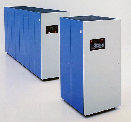
If I remember correctly, I saw a “refrigerator” much like these in the CEC server room at the School of Engineering when I was a student.

By 1987 this more compact little model had the astonishing capacity of 7.5 gigabytes:

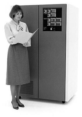
Today, just 24 years later, we have devices like this one:

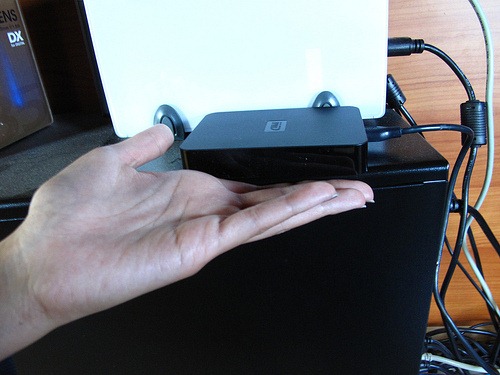
With a capacity of 1 terabyte, about 134 times the capacity of that last one, in the palm of your hand.

Amazing, isn’t it?

Given that we have this much storage capacity, at ever lower cost, it’s only logical that what we want to do is improve our ability to analyze data.

What if we want to do time series analysis, forecasting, the kind of work that groups information sequentially, where order matters? The kind of analysis that answers questions like: what happened? why did it happen? what will happen next?

Storage doesn’t solve this problem; what solves it is software capable of using that capacity intelligently. The traditional answer from a present-day software engineer will be: “store the information in a relational database, because that way you’ll be able to analyze it efficiently and safely.”

But things aren’t that simple.

An exercise in data analysis

I don’t know how much information will be collected in the upcoming 2012 population census, but suppose only the following variables were captured: sex, age, region, level of schooling.

Sex can be stored in 1 bit, age in 7 (let’s assume nobody lives past 127), and there are 16 regions, so that fits in 4 bits. Level of schooling goes from 0 to 12 for the full schooling guaranteed by our constitution; let’s say 13 means vocational or technical education, 14 university, and 15 a graduate degree. All of that fits in 4 bits. So a simple scheme for storing these variables from Chile’s 2012 census is this:

sex: 1 bit age: 7 bits
region: 4 bits
schooling: 4 bits
Total: 16 bits, 2 bytes

Let’s reserve 20 million records: the information fits in less than 40 megabytes. Given what today’s personal computers can do, this demographic information can be held in RAM and used for simple calculations, such as computing the median, for example. On my PC a C++ program (about 70 lines of code) that computes the median age per region takes around 200 milliseconds.

You can store these 20 million records in a relational database. In my case I used SQL Express, and it took me 2 minutes to load all the records from a CSV file.

Computing the mean age is, in programming terms, much simpler. This simple SQL query is enough:

select region, sexo, avg(edad) from datos_censo
group by region, sexo
order by sexo, region

This calculation takes 7 seconds, about 30 times longer than my C++ program. Of course, the mean is not the same thing as the median. Unfortunately Transact-SQL has no median function, so to do the same thing as my C program you have to write an ugly SQL statement¹.

All these exercises have used a very simple database, with barely 3 variables. If the census measured some 200 variables, and we used 2 bytes for each possible value, the entire census would take up about 7.5 GB. The census data could be processed on a laptop.

Reality isn’t that simple, because the big problem is collecting the information and keying it in, in a distributed fashion, at data collection centers in different parts of the country, with hundreds of census takers who will have to enter the data, and so on. All of this will require adequate infrastructure, with backup systems; it will surely be published online and hosted in a data center, and maintaining that infrastructure will carry an extravagant cost computed by the enigmatic calculators of the data center’s sales executives.

The census IT team will probably create a pretty relational model to organize the information, trying to keep it in at least third normal form, in order to improve transaction times when the data is entered (besides the census data, you need administrative and control data to guarantee the integrity of the information). But after all those complications, the information can perfectly well be dumped into a vector, a single table with one field per variable and some 20 million rows, and be processed efficiently to compute a whole range of statistical indicators. I wonder whether they’ll do it that way, or turn to SQL for these calculations.

While I was writing this post, SQL Server on my computer tried to compute the median age of the 20 million simulated records. Let me remind you that my C++ program took 230 milliseconds. The SQL statement was interrupted after half an hour; analysis of the execution plan reveals that the table scan and the subsequent join will mean going through 400 trillion rows. Adding indexes won’t solve the problem², and their impact will probably be minor. The solution in these cases is to write a stored procedure, or to walk the data with cursors, a task of programming complexity similar to my C++ algorithm, and, I suspect, with worse results in time (the reader could try to solve this problem with another relational database, or program the median calculation in Transact-SQL).

The problem with relational databases

This is a simple problem, with just one table, and with an amount of data that isn’t that large by today’s standards. There are applications that are much bigger. At my job we have databases with hundreds of gigabytes of information, which pose challenges well beyond this one.

The thing is that relational databases are very efficient at processing transactional operations, the kind that add, insert, retrieve and modify a small amount of data in a much larger database.

Picture a typical transactional shopping website: a user logs in to the site, the account information is retrieved, session data is written to a log, products are searched, a purchase order is created, the user’s data is updated, payment is recorded, and so on. Thousands of transactional operations, but each one handling a subset of the total data.

Over time this database will hold billions of records, and at that point the sales department will need to analyze that information. When we try to meet those needs with SQL we’ll run into problems similar to the ones I faced with my little census data exercise. We’re looking at the classic change of approach: we go from the transactional world, where relational databases reign, to the problem of massive processing (1 out of 5,000 is not the same as 5,000 out of 1).

What does it mean to process a large amount of data?

Not long ago I solved a similar problem at work. In one part of a process carried out by a group of analysts, 70,000 vectors had to be sorted using Microsoft Excel. They had built the process themselves because there is still no application for this service. The problem was that this sort took 4 hours for those 70,000 vectors, and there are files of up to 400,000 vectors to process (yes, it can be done with Excel, a big machine and a lot of patience). Rewriting the vector sort in C took 1 hour, and it does the calculation in under 1 second for the 70,000 vectors, on a PC. The bottleneck in the process disappeared.

Not that many years ago no business analyst would have tried to solve this problem with Excel. The capacity simply wasn’t there; it was considered a large-scale problem that required custom development by the IT department. In the 90s that would have been a big data problem.

What is big data? That is the question Adam Jacobs asks in his 2009 ACM Queue article: “The Pathologies of Big Data”. What are we talking about? Gigabytes? Terabytes? Petabytes? Jacobs proposes the following meta-definition:

“data whose size forces us to look beyond the tried-and-true methods that are prevalent at that time.” In the 1980s, it was data sets so large that they required a robotic “tape monkey” to swap thousands of tapes in and out. In the 1990s, perhaps, it was data that went beyond the limits of Microsoft Excel and a desktop PC, requiring analysis software written for Unix workstations. Nowadays, it may mean data that is too large to be placed in a relational database and analyzed with the help of a desktop statistics or data visualization package, data whose analysis requires massively parallel software running on tens, hundreds, or even thousands of servers.

Those are the problems we face now. Our users have access to hardware able to store huge amounts of data, capacities that were unthinkable just two decades ago; what they need are software solutions that let them work with that data efficiently. That is the challenge, and the tools the market offers, or sets as standards, are not up to this new reality.

Fortunately a mix of old techniques and a few innovations, plus what current hardware makes possible, is enabling the construction of new tools that can meet these demands. That is something we’ll explore in the next few articles.